Portfolio Optimization
Table of Contents
Intro
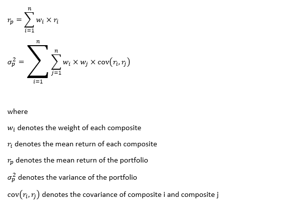
When we talk about trading, we always discuss optimal entry and exit points. We rarely speak of portfolio construction, which is equivalently important as entry signal to your return, if not more. As the old saying goes, don't put all the eggs into one basket. Asset diversification is the best way to reduce systematic risk and idiosyncratic shock. Diversified allocation insulates your entire portfolio from the ups and downs of a single stock or class of securities. For those of you who study finance, modern portfolio theory is the ideal mathematical framework for assembling a portfolio of assets such that the expected return is maximized for a given level of risk. However, I watched a video by Wolfram recently. It challenged the traditional approach and introduced graph theory to portfolio optimization. There are plenty of quant shops deploying fancy mathematic tools to solve the market. The real question for us is, as fancy as it sounds, does graph theory work on portfolio optimization?
Degeneracy Ordering
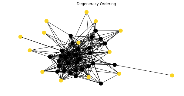
To construct a graph ADT, we need vertices, edges and weights. Let’s take Euro Stoxx 50 Index from 2014 to 2018 for instance. We take 60/40 split and set 2014 to 2016 as the training horizon, 2017 to 2018 as the testing horizon. We denote 50 composites as the vertices. We denote the correlation between the mean return of two stocks as the weights. Only if the correlation exceeds the preset threshold (0.6 in this case), we establish an undirected edge between two vertices.
Inevitably, there may be some individual stocks that have no correlation larger than 0.6 with other stocks. These are very important outliers. As the objective is to diversify our investment, the smaller the correlation we have, the better diversified portfolio it is. If outliers have zero correlation with other strongly connected components, we will have independent stocks that do not suffer from spillover effect. If outliers have negative correlation with other strongly connected components, it is even better, we will have negative correlated assets to hedge against the market turmoil.
These outliers are listed below.
- Adidas AG
- ASML Holding NV
- Amadeus IT Group SA
- Koninklijke Ahold Delhaize NV
- Nokia Oyj
- Vivendi SA
Apart from the outliers in the graph ADT, there is another important part. Even inside strongly connected components, we can still select assets that are not highly correlated with each other. In graph theory, we call these vertices, independent vertex set. An independent vertex set is a subset that no two vertices of which are adjacent. Usually, there are more than one maximal independent vertex set, what are our selection criteria?
Here, we borrow a concept from K-core, degeneracy ordering. Degeneracy ordering is to repeatedly find and remove the vertex of smallest degree from the graph ADT. The degeneracy is then the highest degree of any vertex at the moment it is removed. To find our optimal independent vertex set, the process is illustrated below.
- Get degeneracy ordering in linear time (Matula and Beck, 1983).
- Choose the vertex with the lowest order.
- If the selected vertex is not adjacent to any other vertices in the output set, append the selected vertex.
- Repeat step 2 and step 3 until all vertices have been examined.
The figure below has identified our independent vertex set from the graph ADT.
The independent vertex set contains the companies below.
- CRH PLC
- Deutsche Boerse AG
- Fresenius SE & Co KGaA
- Intesa Sanpaolo SpA
- Kering SA
- Linde PLC
- Orange SA
- SAP SE
- Safran SA
- Sanofi SA
- TOTAL SA
- Unilever NV
- Vinci SA
- Volkswagen AG
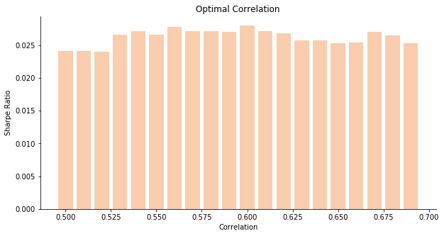
You may argue why we ignore correlation smaller than 0.6. If we iterate different possible numbers from 0.5 to 0.7, the empirical result will tell 0.6 is indeed the optimal threshold for correlation. When the threshold is set at 0.6, we assign equal weight to our independent vertex set plus outliers to construct a new portfolio called Degeneracy Index. The new portfolio at 0.6 yields the largest Sharpe Ratio among other scenarios.
Clique Centrality
The second idea is the reverse of diversification. We try to seek the highly concentrated asset combination to replace the benchmark Euro Stoxx 50 Index. Assuming the removal of unnecessary assets could boost the return, we focus on several individual stocks instead. To select the highly correlated asset combination, we have to propose a relatively advanced concept - cross maximal clique centrality. The centrality is defined as followed. The number of maximal cliques that contain the given vertex is the cross maximal clique centrality of the given vertex. The intuitive rationale is straight forward. The vertices frequently appear in many maximal cliques must be the most influential. In general, it appears that clique centrality indicates embeddedness in dense regions of a graph ADT (Everett and Borgatti, 1998). In CytoHubba, this centrality is simply called Maximal Clique Centrality.
The process of extracting concentrated combination is listed below.
- Iterate all maximal cliques via Bron-Kerbosch algorithm.
- Compute cross maximal clique centrality for each vertex.
- Select vertices where its cross maximal clique centrality is larger than the preset threshold.
The distribution of cross maximal clique centrality indicates 10 is not a bad choice for the threshold.
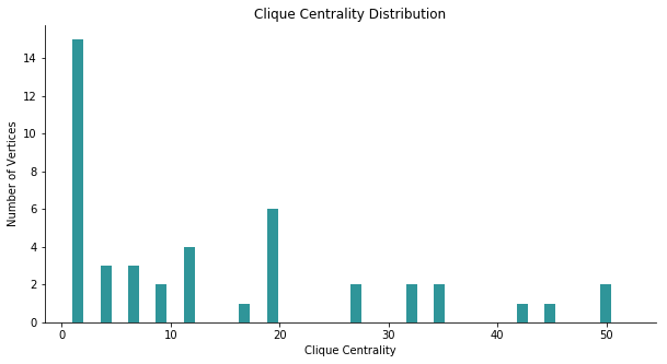
By setting the threshold at 10, we are able to obtain our highly concentrated combination as below. We assign equal weight to each composite to construct a new portfolio called Clique Index.
- AXA SA
- Air Liquide SA
- Allianz SE
- BASF SE
- BNP Paribas SA
- Banco Bilbao Vizcaya Argentaria SA
- Banco Santander SA
- Bayer AG
- Bayerische Motoren Werke AG
- Daimler AG
- Deutsche Post AG
- Deutsche Telekom AG
- Enel SpA
- Engie SA
- Eni SpA
- ING Groep NV
- Industria de Diseno Textil SA
- Schneider Electric SE
- Siemens AG
- Societe Generale SA
- Telefonica SA
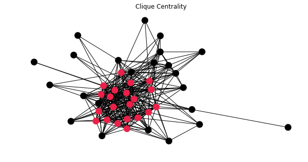
The figure below has implied our combination located at the very core of graph ADT.
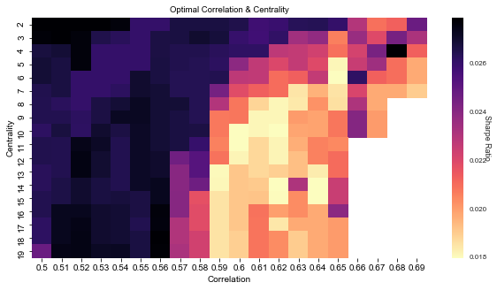
To find the optimal thresholds for both correlation and cross maximal clique centrality, we apply brute force calculation to try correlation from 0.5 to 0.7 and centrality from 2 to 20. To achieve the maximum Sharpe Ratio, the best thresholds seem to be 0.5 and 2 for correlation and centrality.
Markowitz Optimization
Modern portfolio theory was introduced in 1952 by Nobel laureate Harry Markowitz. The idea was to find the asset allocations that provide the lowest possible risk for any level of expected return. There are three possible types of strategy when it comes to portfolio optimization.
- Maximize Sharpe Ratio
- Minimize variance
- Maximize return
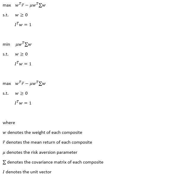
To maximize Sharpe Ratio, we should recall Lagrangian multiplier from calculus. Here, the Lagrangian multiplier is called risk aversion parameter, it denotes the risk aversion level of the investor. To make our lives easier, we set the parameter at 1. For those of you who are familiar with convex optimization, this equation is called linear programming with random cost. We will use the package cvxopt to solve such a problem. You can see the example of quadratic programming. The following equations are presented in matrix form.
With the result of cvxopt.solvers.qp, we assign weights accordingly to construct Sharpe Index, Variance Index and Return Index. Strangely enough, the weights to maximize Sharpe Ratio are very similar to the weights to maximize the return.
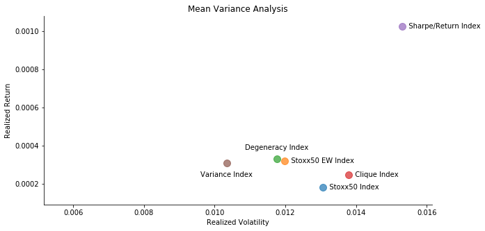
For in-sample data comparison, we also introduce another benchmark, Euro Stoxx 50 Equal Weight Index. Believe me 🤦-2642; this product really exists! We bring all indices to the mean variance analysis to evaluate its performance. It seems that Sharpe/Return Index (since they are very similar so we put them together) always outperforms the rest. It is quite normal because these two indices seek the local maximum of our given function. Surprisingly, Stoxx50 EW Index always outperforms the actual Stoxx50 Index. The actual Stoxx50 Index is computed via Laspeyres formula. Given the consideration of market cap and share liquidity of each composite, Stoxx50 Index leans heavily towards companies with larger market cap and more share liquidity. Commonly speaking, these blue-chip companies are more likely to be correlated to the overall macroeconomic situation. In another word, Stoxx50 Index is designed to leans towards highly correlated stocks. Stoxx50 EW Index seems to be a much better choice when constructing a portfolio. Less correlated stocks have larger weights in the portfolio. In terms of time complexity, Stoxx50 EW Index outweighs any other indices undoubtedly. Degeneracy Index and Variance Index demonstrate the lowest volatility among all. Regarding the linear time complexity of degeneracy ordering, it can be a good approximation to seek for minimum variance portfolio. As for Clique Index, it is the lame duck out of all. It has one of the highest time complexities due to NP-hard clique searching algorithm. It proves the point that asset diversification is necessary.
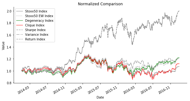
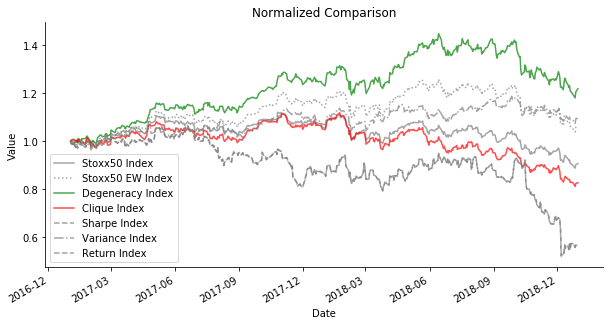
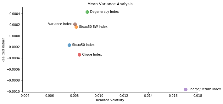
For out-of-sample data comparison, things take a dramatic turn. Degeneracy Index seems to outperform any other indices. The in-sample star, Sharpe/Return Index has the worst performance. Perhaps you think I am cherry-picking. If you change the time horizon of training and testing dataset, you will find that Degeneracy Index always outperforms Stoxx50 Index and Stoxx50 EW Index despite the market sentiment. In a bear market, Sharpe/Return Index is practically useless. It is aligned with the criticism of modern portfolio theory. The historical measurements of asset return and volatility do not translate to the guaranteed performance in the future. They frequently fail at new circumstances, especially something has never occurred in the history. In spite of different ways of train test split, Variance Index and Degeneracy Index are the most consistent performer. The diversification maintains an edge of small volatility even though it suffers from a smaller Sharpe Ratio and return in a bull market.
But if you think I am pitching the application of graph theory to portfolio optimization, you are wrong. I'd love to point out, it's always a good idea to try equal weight first. It is one of the few simple yet effective strategies.
Click the icon below to be redirected to GitHub Repository