Text Mining
Table of Contents
Intro
Is machine learning the best solution to text mining?
What if graph theory beats it in both time and space complexity?
The answer is obvious, absolutely not. When the spotlight shines on machine learning, graph theory is rarely mentioned. First, let's talk about what this project is and later you would realize why sometimes graph theory works better. In this case, graph theory outperforms machine learning in both time and space complexity.
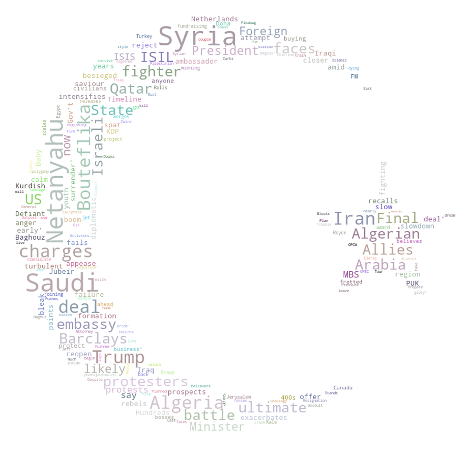
The generation of the word cloud below is done in this script.
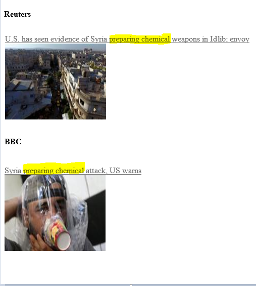
This project is designed to be integrated into my scraping script called MENA Newsletter. Initially, the script would scrape news titles from different mainstream websites (so-called fake news by Mr. Trump 😂 ) including BBC, Reuters, Al Jazeera, etc. All the scraped news titles, links and preview images would be concatenated into one HTML email which is automatically sent to my inbox every morning. After a couple of days of experiments, I realized that many websites were actually reporting the same story but in different titles and preview images. It was totally a waste of energy and time to read these similar contents over and over again. And not every piece of information was worth my time to read. Some stories such as 'British Iranian woman got put in jail' was not exactly business related (I'm sorry, it is a great story though). Couldn't I find a way to create a filter to extract the key information?
Supervised Learning
The first thing came to my mind, of course to anyone, was machine learning. Given the halo around it, we can hardly be blamed. We could build up a classifier to determine which one is key information. A simple Naive Bayes Multivariate Event Model would do the trick. The methodology is basically based on the assumption that when certain key words such as 'crude', 'south pars' and 'LNG' appear together in a title, the title is more likely to be petroleum business related. The model works pretty well for key information screening. The accuracy is always capped at 75 percent. It can be improved by building up a better vocabulary matrix. The downside of the method is the human input. The metadata needs to be manually classified before feeding to the machines. The labor intensity is always the issue of supervised learning.
Still, that doesn’t solve the problem of similar contents with different titles. You may argue we could build up a two-dimensional dataframe with the length of n*(n-1)/2 assuming n is how many titles we have scraped. The purpose is to compare all the titles mano-a-mano to check if they refer to the same story. Surely, we could. Support Vector Machine or Random Forrest or any other supervised learning classifiers can remove the similar contents and extract the key information. All of a sudden, the time and space complexity shoot through the roof. Additionally, the hassle of training metadata just gets doubled.
Unsupervised Learning
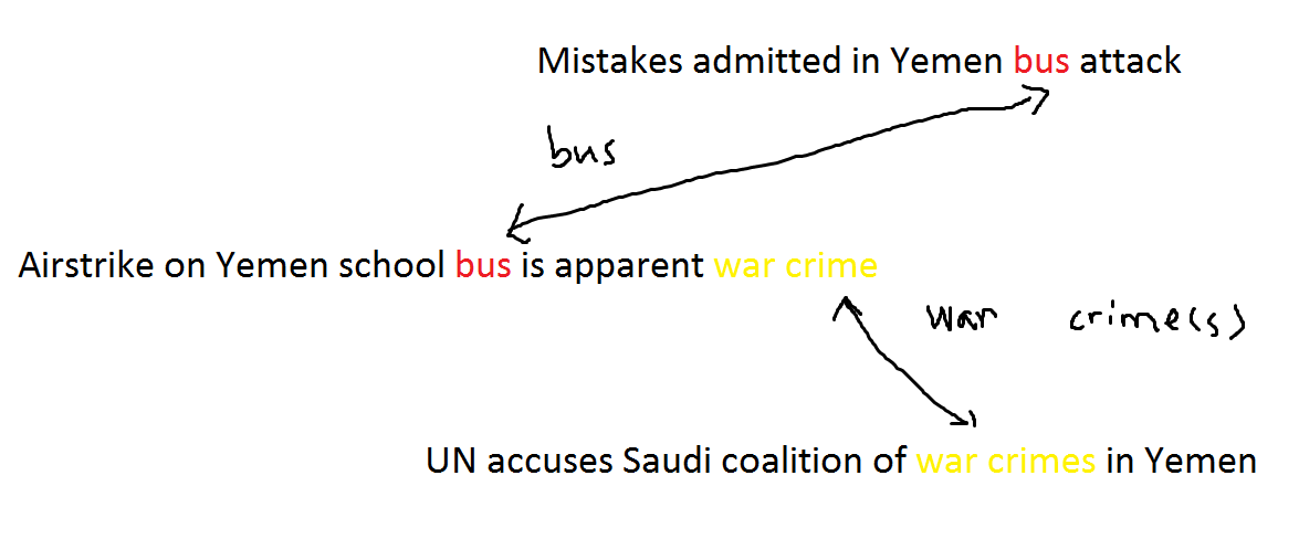
That is not the dead end. Alternatively, we can do an unsupervised learning. How so? Assuming a piece of story is a breaking news, it is so important that every mainstream media would cover it. Maybe different media websites cover the story from different perspectives in relatively different titles. The script called MENA newsletter scrapes a lot of major websites. There must be some overlaps of the stories. Within each story, the titles from different sources should share at least one key word in common. The common key word could be location, event or even name. For example, we have the following titles, 'Airstrike on Yemen school bus is apparent war crime' from CNN, 'UN accuses Saudi coalition of war crimes in Yemen' from Financial Times and 'Mistakes admitted in Yemen bus attack' from BBC. These titles are connected by the common words 'school bus' and 'war crime' ('yemen' is a stop word so excluded). The content 'yemen bus attack is a war crime' exists in every media website under different titles. Apparently, these similar contents should be able to form a cluster.
Yet, there is another problem, how can we compare word 'walking' with word 'walked'? Well, in that sense, we need stemming and lemmatization. Stemming is to revert a word back to its root. Currently NLTK is the most popular NLP package. The famous Porter stemmer is not very effective, as it's a rule-based stemmer. English, unlike its neighbor language Français, has messy vocabulary rules. Because many phrases are stolen from other foreign languages. Keeping a dictionary-based stemmer would require a lot of space. Hence, we would have to cope with the imperfection, which basically means chopping off the end of a word. Lemmatization is to normalize a word back to its base form. It removes all past simple and past participle forms. Wordnet lemmatizer is a relatively better tool than Porter stemmer, even though they both have their shortcomings. In general, I prefer to apply lemmatization before stemming to get a clean vocabulary matrix.
If our assumption holds, we could end up with plenty of clusters inside our text dataset. Each cluster refers to one underlying story. Within each cluster, all the data points (titles) share some common words. Inevitably, there are anomaly data points far from all the cluster. These outliers could be either exclusive content or utterly nonsense. How to deal with them entirely depends on user preference. I personally lean towards false positive. I’d rather have more false positive than false negative for the fear of missing out.
Thus, we shall dig out all the unique stories. We only need a little bit of extra help from the overhyped algorithms, DBSCAN. DBSCAN is a fascinating algorithm. It has the capability of both linear and non-linear classification. It can automatically detect the number of clusters, but it requires a careful tuning of its within-distance parameter, ε. The way I see, this is purely quid pro quod. You can argue OPTICS do not require preset within-distance, but the tradeoff is the greater time complexity (truth is I haven’t updated my sklearn yet :sweat_smile: ). Aside from ε, there is another preset parameter, the minimum sample requirement to construct a cluster. As usual, we always consider the worst case, which is 2. For a clustering problem, the maximum number of clusters you can achieve is n//2 where n is the number of data points. Although setting minimum sample at 2 changes the nature of DBSCAN, the algorithm per se is equivalent to single link hierarchical clustering now. The raison d’être in such an action is that hierarchical clustering is commonly used in NLP for compound identification and extraction.
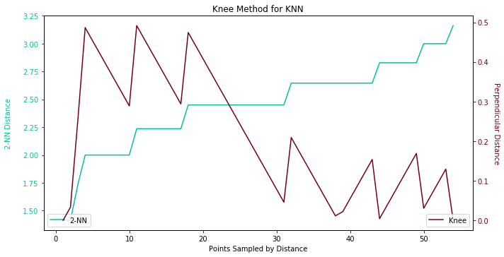
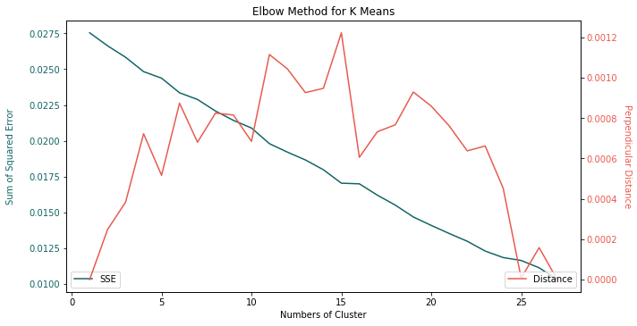
Hereafter, we seek a conventional way to determine the ideal epsilon, K Nearest Neighbors. By using knee method, the optimal ε should occur before the biggest surge on 2-NN distance. By tradition, the selection of K should be minimum sample minus one. Since 1-NN is terribly biased, we go with 2-NN. Unfortunately, we cannot see where the kneecap is in the following figure. We can only tell the number is respectively 2.24 judging by perpendicular distance.
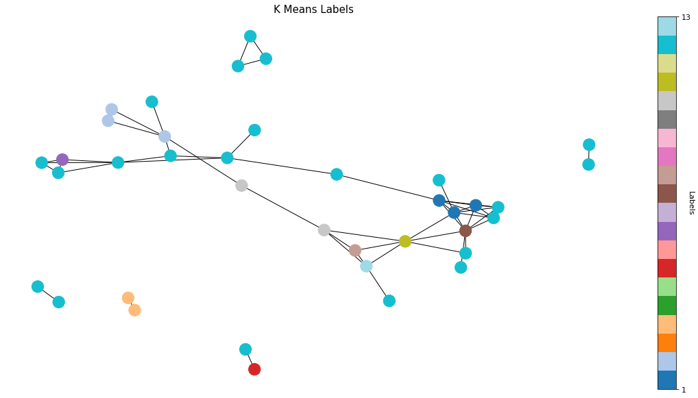
To be honest, the result of DBSCAN comes as a surprise. There are only 3 different labels. If we take a quick scan at the text data, we could certainly identify more than 3 important stories. The frustrating result left us no choice but to pick a naïve unsupervised learning algorithm, K means. Don’t get me wrong, K means is a simple but powerful tool. It is fast and intuitive regardless of its linear boundary. The only fuss is to find the optimal number of clusters. There are a few empirical approaches. In order to keep things consistent with DBSCAN, the elbow method is applied here.
The number of clusters from K means is 14 which sounds more appropriate. The next step is to pick one data point as end result from each cluster. My answer is the randomness. Randomly select a title from each cluster and add to the output. Another way is based upon the source. Some favors Bloomberg, others are obsessed with Wall Street Journal. We can even draw up an order of selection within the cluster. For instance, 3 titles come from Reuters and 2 titles come from BBC within the same cluster. Naturally Reuters gets preferential treatment from this cluster.
Graph Theory
Is that the only trick up my sleeves? Never, I am David Copperfield, I walk through the Great Wall and make Statue of Liberty vanish into thin air. Here comes a great one, how about graph theory? We could connect news titles from different sources on the condition of how many words they have in common. As usual for natural language processing, we always need to keep a stopword list to exclude some stop words. Stopword implies words like 'we are' which is common in sentences but do not have an impact on the outcome of NLP. In our case, some country or city names such as 'lebanon', 'iran', 'tehran' or 'beirut' should be included in the stopword list.
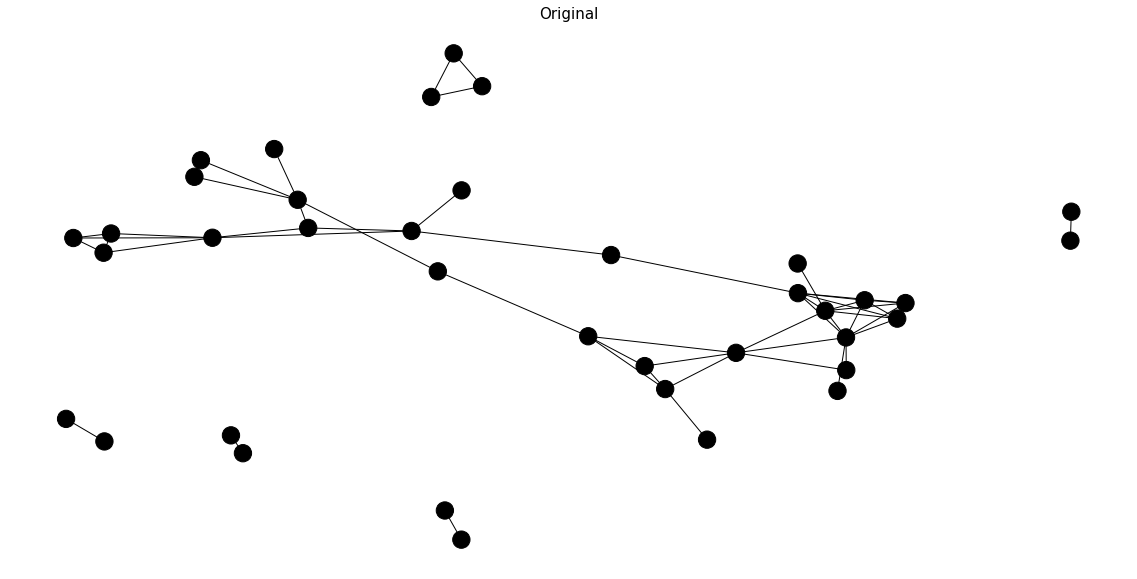
Enough chitchat on the theories, let's visualize the graph network and see what is really happening. The index of the news title in a concatenated dataframe would be presented as the vertex name. Why not the exact titles? They are too wordy. The edge between two vertices would be established if and only if two news titles share some words in common. The number of common words would be denoted as the weight of the edge. Some titles may not have any word in common with the rest. These lone wolves do not appear in this graph structure. Later on, we could add these rebellious titles back to our output. For the moment, we are only concerned with the vertices in the graph ADT.
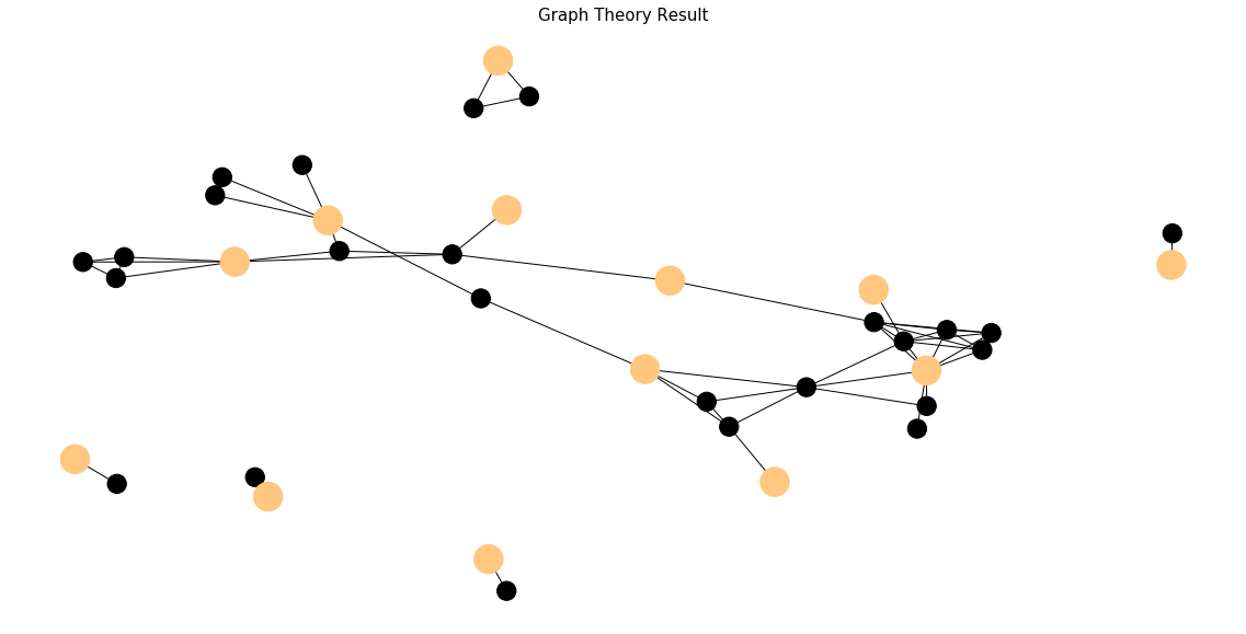
To make graph theory works, the assumptions of unsupervised learning cannot be violated. If one of the stories is important enough, it must have been covered by practically every source. All the titles referring to this story must share some words in common. Translated in graph theory, each story is likely to form a maximal clique. Nevertheless, the maximal clique demands all vertices are connected to each other. In reality, most maximal cliques we can obtain have the order of 2 or 3 which enforces us to make a compromise. Now our target switches to the vertices with abnormally high degree. If you think about it, the vital vertex should connect to all the other vertices inside a subset. Each subset indicates one unique story. All the vertices adjacent to the vital vertex should be redundant as they refer to the same story. Well, degree is not the only valid metric we can rely on. Other metrics such as closeness centrality and eigenvector centrality are available options as long as we can back the assumptions with a reasonable story.
Is there any known traversal algorithm that can return a list of our target vertices? Not to my knowledge (If you do, please feel free to comment). Nonetheless, our selection criteria are not complex and we could always implement our own version of traversal algorithm. Borrowing some ideas from an algorithm to find k-core (Matula and Beck, 1983), we shall easily achieve the objective in linear time.
- Create an ordered dictionary where vertex is the key and degree is the value
- In each iteration, remove the vertex V with the highest degree from the current ordered dictionary
- Append the vertex V into the result set
- Remove all the neighbors of vertex V from the current ordered dictionary
- Repeat step 2 to 4 until the ordered dictionary is empty
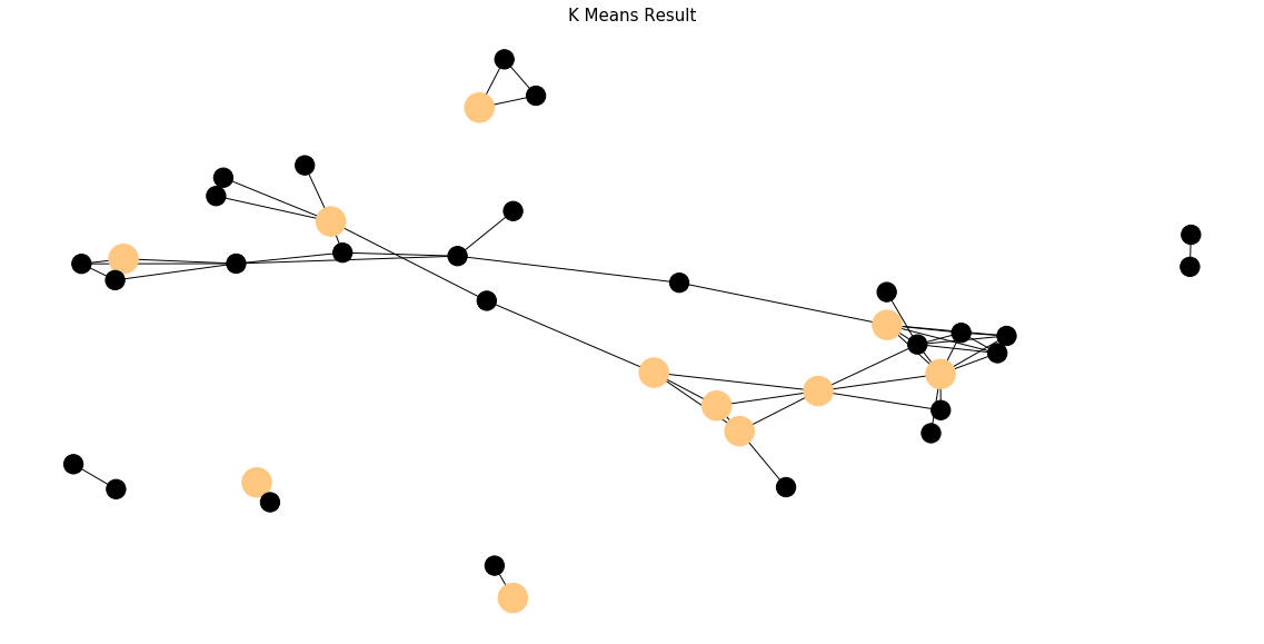
The result turns out to be a huge success. The algorithm gracefully captures all the essential vertices. All the light-colored vertices are selected. All the dark-colored vertices are removed.
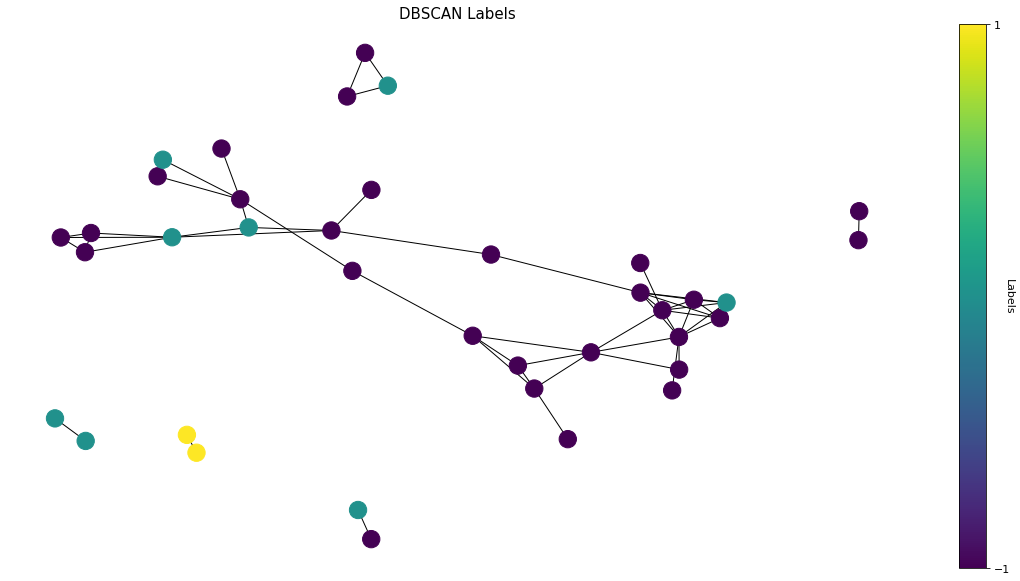
To make comparison, we visualize the output of unsupervised learning in the same graph structure. Frankly I am overwhelmed by the classifications of DBSCAN. Three different labels are mapped by different vertex colors. We can barely find any pattern within the same cluster either by graph theory or by reading through the titles.
K means demonstrates a great solution to our text mining problem. It recognizes some of the strongly connected components inside a graph structure. Though it still seems obsolete against the performance of graph theory. Some of the weakly connected components are misclassified.
The accuracy of the algorithms is a subjective matter. Different people have different opinions on which titles are more important. The evaluation of the accuracy is a state of art. Estimating the accuracy of machine learning in a graph theory framework is sort of unfair. However, the time and space complexity of algorithms are an objective evaluation. Leveraging the inline magic of iPython, %timeit, the argument of graph theory supremacy is loud and clear. Graph theory takes 104 ms ± 1.93 ms per loop while K means is running 3.98 s ± 28.6 ms per loop. The time complexity of a standard K means is O(k*n*d), where k is the number of clusters and d is the dimension of the dataset. Don’t forget the elbow method. It requires us to try a few times of K means to find the optimal number of clusters. On the contrary, the graph theory approach is merely O(n). The king of space complexity goes to machine learning without saying. Let’s take a look at auxiliary space. A large feature vector is unavoidable for natural language processing. Assuming we have N sentences, each sentence involves 5 unique words, 2 shared words and 1 stop word. The vocabulary matrix is going to be (5*N+2)*N. In contrast to machine learning, a graph structure can be represented by an N by N adjacency matrix where N is the order of the graph. The adjacency matrix can be further shrunk to adjacency list if facing a sparse graph.
Finally, is this approach flawless? Nope. As George Box(a statistician, his Box-Jenkins method is the foundation of time series analysis) said,
All models are wrong, but some are useful.
As much as I love the algorithm I developed, it could still miss some information. Consider we have two vertices, 'Nazanin Zaghari-Ratcliffe back in Tehran prison' and 'Some 400 prisoners escape prison in Tripoli chaos'. They are connected by the common word 'prison' but they appear to be completely different stories. We may exclude a false negative by accident. Is there any room for improvement? Yes and always. Currently we assume what we scrape is the latest news from different sources. Any involvement of historical archives requires an introduction of a new dimension, time, into the graph structure. Our edge connection based upon common words may sabotage the news timeline without precaution.
In short, graph theory is a better approach for our text mining problem. It answers the question at the very beginning, machine learning is no silver bullet. Graph theory is severely underestimated amid the full publicity of machine learning.
Click the icon below to be redirected to GitHub Repository